MinHash & LSH
Background
In my previous post I explained how the MinHash algorithm is used to estimate the Jaccard similarity coefficient, because calculating it precisely each time can be expensive. However, we still need to compare every document to every other document in order to determine which documents are similar (or in more fancy words - to cluster the documents by similarity).
Doing that has a time complexity of $O(n^2)$, where n is the number of documents we’re comparing.
We can optimize this process by using the concepts of Locality-sensitive hashing (LSH).
As always, in order to get something we need to give something, this time the trade-off is between accuracy and performance. Meaning that we’ll get a much better performance (time complexity), but we’ll pay with a bit less accuracy (and like before, we can estimate our “mistake” probability).
The General Idea
Let’s say that we consider two documents to be similar if their Jaccard similarity coefficient is greater than 0.9 (more than 90% similar). Given a new document D, we need to compare it to every other document to determine whether there exists one that is similar (>90%) to our new document D.
But there might be some documents that by briefly looking at their minimum hash values, are most probably going to be less than 90% similar to this one, so we might want to take the chance and avoid comparing those to our new document D. Saving us time, but taking the risk of missing out on a potential similar document.
This is the general idea of how we’re going to use the conecpts of Locality-sensitive hashing with the MinHash algorithm.
The Technical Details
Using the MinHash algorithm, we choose some value k to be the number of hash functions we’re going to use. So for every document we process, we need to calculate k minimum hash values ($h_{min}(D)$).
We will call them from now on the MinHash values of the document.
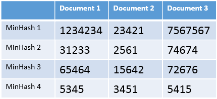
Next we need to create a table that has the n documents as its columns and the k MinHash values as its rows, as can be seen in this example:
Last thing we need to do, is divide this table into b bands, each one consisting of r rows, so that $b*r=k$. For example, if we are using 12 hash functions (our k value), we can split the table into 4 bands (our b value) with 3 rows each (our r value), ending up with 4 tables that look something like this:
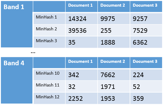
Now when a new document D arrives, and we want to determine whether there exists another document that’s similar to it, we will go over every such band, and look for documents that share the exact same MinHash values on every row of that band. If such document exists, then we’ll do the full MinHash comparison between this document and the new document D.
For example, if the new document has MinHash values of 7662, 1971, 1953 on rows 10 to 12, then we’ll do the MinHash comparison between this new document and document 2, since they share the exact same values on band 4.
And what if a new document shares no identical rows to any other document on any band? In this case we assume that there exists no similar document to it.
Note that we did that without actually doing any MinHash comparison.
So to recap, we only compare two documents if there exists a band where those two documents share the same values on every row.
Therefore, our goal is to find a division into rows and band such that if two documents are not compared (share no band), the probability of them actually being similar is very low.
Choosing the right number of rows and bands
Before I can show you how to choose r (rows) and b (bands), we first need to crunch some numbers:
- Recall that the probability of two documents having the same MinHash value on any row is exactly $J(A,B)$, and every row is independent of the other.
- The probability that two documents have the same MinHash values on all rows of a given band is therefore $J(A,B)^r$
- The probability that two documents have at least one different MinHash value on any row of a given band is the complementary of the previous step $1-J(A,B)^r$
- The probability that two documents have at least one different MinHash value on any row of any band is $(1-J(A,B)^r)^b$
- The probability that two documents have the same MinHash values on all rows of at least one band is $1-(1-J(A,B)^r)^b$
After all this hard work, step 5 describes the probability that we’ll need to do the MinHash comparison on two given documents:
$\Pr(\text{Do MinHash compare on A and B}) = 1-(1-J(A,B)^r)^b$
It might be hard to see, but on the interval of $J(A,B)\in[0,1]$ the graph of this probability function is going to look something like this:
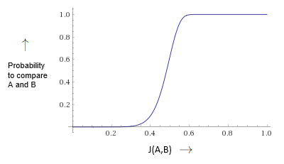
This kind of graph is called an s-curve graph, and it’s special because its values are very low until it reaches what’s called a step and then its values quickly increase and stay very high.
We can utilize this property to our advantage, by making sure the step occurs as close to the threshold (of two documents being similar), as we can.
Luckily, we can estimate the step with an equation that’s based on r and b, and this will be our key to determining what values of r and b to choose:
$\text{step} \approx \Big(\dfrac{1}{b}\Big)^{\tfrac{1}{r}}$
For example, let’s say that we consider two documents to be similar if their Jaccard similarity coefficient is greater than 0.9 (more than 90% similar), and we used 400 hash functions in our MinHash implementation.
We want our step to be as close to 0.9 as possible, so we choose to divide our 400 hash functions value to 20 rows and 20 bands, giving us a step value of $\Big(\dfrac{1}{20}\Big)^{\tfrac{1}{20}}\approx 0.86$
So we end with this nice probability table:
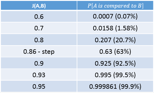
In this table we can see that if the Jaccard similarity coefficient of two documents is lower than 0.8, it is highly unlikely that we’ll end up doing the MinHash comparison on them.
But, if the Jaccard similarity coefficient of the documents is greater than 0.9, then we’re most probably going to do the MinHash comparison on them, and thus find out that they are indeed similar.
In conclusion, we’ve seen that we can avoid doing the MinHash comparison on a lot of documents, and still get the right results with a very high probability.
This is of course not a bulletproof method, and you might end up classifying documents that are similar as dissimilar, but this is ok as long as we can tolerate an occasional error.
You can see a full example of the MinHash implementation with LSH optimizations, on my GitHub page:
Java implementation
C# implementation
Python implementation
Step Approximation Proof
I’ve been getting requests to prove that the step of the probability function of comparing A and B is approximately $\Big(\dfrac{1}{b}\Big)^{\tfrac{1}{r}}$
To do that, let’s first rewrite that probability function in terms of x and f(x), where x is J(A,B):
$f(x)=1-(1-x^r)^b$
Three things to notice about this function:
- $x=0 \to f(x)=0$
- $x=1 \to f(x)=1$
- $x\in (0,1) \to 0\lt f(x)\lt 1$
In order to get a better understanding of how f(x) increases from 0 to 1, we’ll differentiate it:
$\dfrac{df}{dx}(x)=br(1-x^r)^{b-1}x^{r-1}$
Since b and r are always positive integers we can see that:
- $x \in (0,1) \to \dfrac{df}{dx}(x) > 0$
- $x=0 \lor x=1 \to \dfrac{df}{dx}(x)=0$
From note 1 we know that the derivative function is always positive so this means that our original function f is a monotonically increasing function in the range of $x \in (0,1)$.
By adding note 2 we know that the derivative function should have a maximum value in this range (Extreme Value Theorem).
This maximum value is where the original function f increases the fastest, or in other words, where its slope is the steepest. We can find this maximum point by differentiating again:
$\dfrac{d^2 f}{dx^2}(x)=br(1-x^r)^{b-2}x^{r-2}\Big((r-1)-(br-1)x^r \Big)$
This equation might look scary, but we’re looking for the points where $\dfrac{d^2 f}{dx^2}(x)=0, x \in (0,1)$ so we can divide a lot of terms and end up with this x value:
$\dfrac{d^2 f}{dx^2}(x)=0 \to x^r=\dfrac{r-1}{br-1} \to x=\Big(\dfrac{r-1}{br-1}\Big)^{\tfrac{1}{r}} \to x=\Big(\dfrac{1-\frac{1}{r}}{b-\frac{1}{r}}\Big)^{\tfrac{1}{r}}$
We only found one critical point (the maximum point), which means that the first derivative should look similar to a parabola, and this is enough to deduce that our original function f will be an s-curve function. Therefore, the maximum point we’ve just found is also where the step occurs. All that’s left to do is get rid of some $1/r$ values that don’t change much and end up with this equation:
$\text{step} = \Big(\dfrac{1-\frac{1}{r}}{b-\frac{1}{r}}\Big)^{\tfrac{1}{r}} \approx \Big(\dfrac{1}{b}\Big)^{\tfrac{1}{r}}$
Error Analysis
Before we wrap things up, let’s do a quick error analysis to get an idea of how likely we are to make mistakes using this method.
False Positives - Given a new document that’s dissimilar to all others, how likely are we to classify it as similar?
In this case there’s 0% chance of making a mistake because even if we do decide it’s likely to be similar to another document, we’ll do the actual MinHash comparison between the two to be sure, and therefore will end up knowing they’re indeed dissimilar.
False Negatives - Given a new document that’s similar to at least one other document, how likely are we to classify it as dissimilar?
This case is equivalent to the probability of not comparing the new document to any other document that’s similar to it.
Let’s say A is our new document, and for now, we’ll look at one particular B that is similar to it.
$\Pr(\text{A and B are not compared}) = 1-\Pr(\text{A and B are compared}) = (1-J(A,B)^r)^b$
Since A and B are similar, their Jaccard similarity coefficient is at least the step (this is how we choose the step):
$\Pr(\text{A and B are not compared}) = (1-J(A,B)^r)^b \leq (1-step^r)^b$
Do some algebra on the step to get:
$\text{step} \approx \Big(\dfrac{1}{b}\Big)^{\tfrac{1}{r}} \to step^r \approx \dfrac{1}{b}$
Put the above equation into our inequality to get:
$\Pr(\text{A and B are not compared}) \leq (1-step^r)^b \leq \Big(1-\dfrac{1}{b}\Big)^b \leq \dfrac{1}{e} \approx 0.37$
This bound is very promising since it means that even if there’s only one such B that’s similar to A, and even if their Jaccard similarity coefficient is very close to the threshold (close to being dissimilar), it’s still more likely (at least 63%) that we’ll compare A and B and find out that they’re similar, than to avoid comparing them and get a False Negative.
And what if there is more than one document that’s similar to A?
Let’s assume that there are $n$ documents that are similar to A and are independent of one another.
We get that the probability of a False Negative decreases exponentially:
$\Pr(A\text{ is not compared to any similar }B_i) = \textstyle\prod_{i=1}^n \Pr(A\text{ is not compared to }B_i) \leq \Big(\dfrac{1}{e}\Big)^n$